Conditional Formatting Not Working in Google Sheets? 3 Silent Mistakes
Your conditional formatting rule looks right, but it colors the wrong cells, only one column, or nothing at all. Google Sheets doesn't show an error when a custom formula is wrong, so these mistakes are silent. We reproduced the most common ones on a task list with checkboxes, where the goal was to cross out every row whose box is ticked.
Only one column changes: the missing $
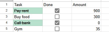
=B2=TRUE, only column A is crossed out.The rule applies to A2:C5 with the custom formula =B2=TRUE. Sheets writes the formula for the first cell (A2) and shifts it for every other cell, just like copying a formula. So in column B the rule checks C2, and in column C it checks D2, which are never TRUE.
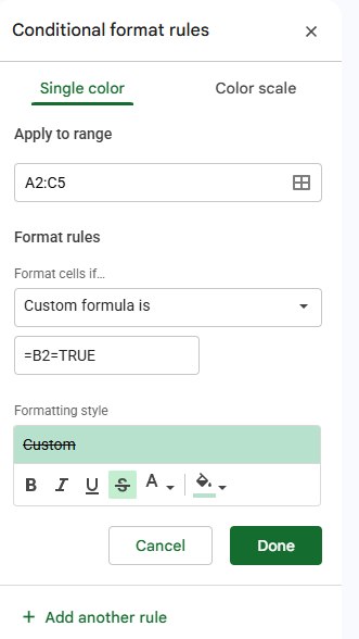
Fix: lock the column with a dollar sign: =$B2=TRUE. The column stays B for every cell, while the row still moves down.
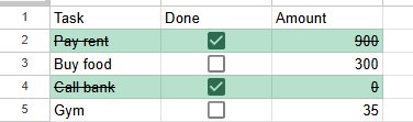
=$B2=TRUE, the whole row is formatted.The wrong rows change: the formula starts on the wrong row
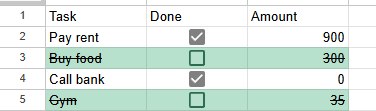
=$B1=TRUE, each row looks at the row above it.Here the rows below the ticked ones were crossed out. The range starts at row 2, but the formula points at row 1 (=$B1=TRUE), so every row checks the box one row up.
Fix: the row number in the formula must match the first row of Apply to range. Range A2:C5 → formula with row 2. If you change the range to start at row 1, change the formula too.
Nothing changes: the formula doesn't start with =
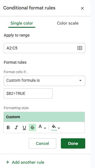
$B2=TRUE without the leading =: no cell was formatted, and no warning appeared.A custom formula must start with =. Without it, Sheets doesn't complain; the rule simply matches nothing. In our test, every row went back to plain text as soon as we removed the =.
Fix: add the = at the start: =$B2=TRUE.
Other things to check
- The range. Look at Apply to range: new rows below it aren't covered. Extend it, for example to
A2:C1000. - Text vs numbers. A rule like Greater than 100 can skip numbers stored as text. If they're left-aligned, convert them first: see SUM not working.
- Several rules on the same cells. Open Format → Conditional formatting with a cell selected to see every rule that applies to it, and remove the ones you don't need.
Frequently asked questions
Why doesn't Sheets show an error for a wrong custom formula?
Because a formula that is valid but never TRUE is a legitimate rule. Sheets only knows the rule matched nothing, not that you meant something else. That's why it's worth testing a rule on a row where you know the answer.
Can I color a row based on text instead of a checkbox?
Yes, with the same $ trick: =$C2="Done". More examples in how to color cells based on value.
How do I cross out a row when a box is ticked?
That's exactly the fixed rule above, with the strikethrough style. The full walkthrough is in how to add checkboxes.