How to Add a Calculated Field to a Pivot Table in Google Sheets (and Get the Right Totals)
A calculated field adds a column to a pivot table that doesn't exist in your data, like Revenue = Units × Price. It's easy to add, but in our test the obvious setup gave wrong totals without any warning. Here's how to add one, why the numbers can be off, and the formula that gave the right result.
Add a calculated field
Our data has Region, Product, Units and Price for five sales, and a pivot table with Region in Rows.
- Click inside the pivot table to open the Pivot table editor (or use the Edit button under it).
- Next to Values, click Add and choose Calculated field at the top of the list.
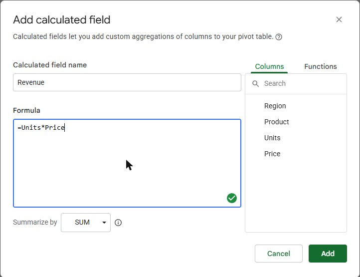
- In the Add calculated field window, give it a name (Revenue) and type the formula using the column names, for example
=Units*Price. A green check means the formula is valid. - Click Add.
Why the totals can be wrong
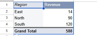
North had two sales: 10 units at 2 and 5 units at 4, so the revenue is 10×2 + 5×4 = 40. The pivot table showed 90. That's 15 (total units) × 6 (total of the prices): with Summarize by: SUM, the formula multiplied the sums of the columns instead of multiplying row by row and adding up. The grand total, 588, was just as wrong (the real total is 118).
East looked right (14) only because it had a single sale. That's what makes this mistake easy to miss: small groups come out correct.
Switching to Summarize by: Custom with the same =Units*Price didn't help either: North showed 20, the first sale only.
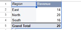
=Units*Price: each group only uses its first row.The fix: Custom + SUMPRODUCT
To multiply row by row and then add, use SUMPRODUCT with Summarize by: Custom:
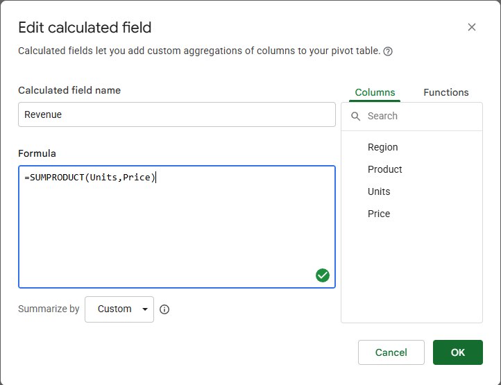
=SUMPRODUCT(Units, Price)- In the editor, click the pencil next to the calculated field's formula.
- Replace the formula with
=SUMPRODUCT(Units, Price). - Check that Summarize by says Custom, and click OK.
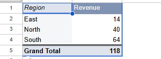
The same rule applies to any calculated field that multiplies or divides two columns: build the per-row calculation inside SUMPRODUCT (or another function that works on whole columns), and use Custom.
"Unknown column name"
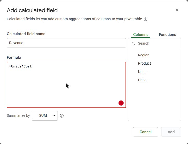
A column name that doesn't exist in the source data turns the formula box red, shows "Unknown column name: 'Cost'" and greys out the Add button. Click a name in the Columns list on the right to insert it exactly as Sheets expects. If a name has spaces, wrap it in single quotes: ='Unit price'.
Frequently asked questions
Is a calculated field better than a helper column in the data?
A helper column (for example =C2*D2 next to your data) is simpler and easy to check row by row. Then you add it to Values with a normal SUM. Use a calculated field when you can't or don't want to change the source data.
How do I group or sort the pivot table?
See how to make a pivot table, including grouping dates by month.