How to Make a Pivot Table in Google Sheets
A pivot table turns a long list into a short summary without a single formula. Total sales per region, expenses per category, orders per month: you drag a few fields into place and Google Sheets does the grouping and adding for you.
Create a pivot table
- Click any cell inside your data. The table needs a header row, with one column per field (for example Category, Item, Amount).
- Go to Insert → Pivot table.
- Check the Data range, choose New sheet, and click Create.
Sheets opens a new tab with an empty pivot table on the left and the Pivot table editor on the right.
Add rows and values
- Next to Rows, click Add and choose the field to group by, for example Category.
- Next to Values, click Add and choose the field to total, for example Amount.
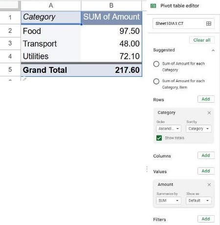
The editor also shows Suggested pivot tables at the top, such as "Sum of Amount for each Category". Clicking one builds the same table in one step.
That's it. Each category appears once, with its total next to it, and a Grand Total at the bottom.
Change SUM to COUNT, AVERAGE and more
In the Values section, open the Summarize by list under your field (Summarise by if your Google account uses UK English) and pick another calculation:
| Summarize by | Answers the question… |
|---|---|
| SUM | How much in total per group? |
| COUNTA | How many rows per group? |
| AVERAGE | What's the typical amount per group? |
| MAX / MIN | What's the biggest or smallest per group? |
You can add the same field to Values twice, for example once as SUM and once as COUNTA, to see the total and the number of purchases side by side.
Add columns and filters
- Columns: add a second field here to make a grid, for example categories down the side and months across the top.
- Filters: add a field to include only some values, for example only this year's rows.
Keep the pivot table up to date
Pivot tables update automatically when the source data changes. If you add rows below the original range, open the editor and extend the data range, or use an open-ended range like Expenses!A1:C from the start.
Tip: you can't type inside a pivot table. To change the numbers, edit the source data. To reuse the results elsewhere, copy them and use Edit → Paste special → Values only.
Frequently asked questions
Where did the Pivot table editor go?
It only shows while a cell in the pivot table is selected. Click any cell of the table and it reappears (look for the Edit button if it stays hidden).
Why does my pivot table show a blank row?
The data range includes empty rows. Tighten the range, or add a filter on the Rows field to exclude (Blanks).
Is there a formula alternative?
Yes. SUMIF gives totals per category, and the QUERY function can group and sum in one formula.