How to Alternate Row Colors in Google Sheets
Alternating row colors (also called banding or zebra stripes) make long tables much easier to read: your eye can follow a row across the screen without jumping to the one below. Google Sheets has a built-in tool for it.
Add alternating colors
- Select your table, including the header row.
- Go to Format → Alternating colors (Alternating colours if your account uses UK English).
- A panel opens on the right. Pick one of the Default styles, or set your own colors under Custom styles.
- Keep Header ticked if the first row is a header, and click Done.
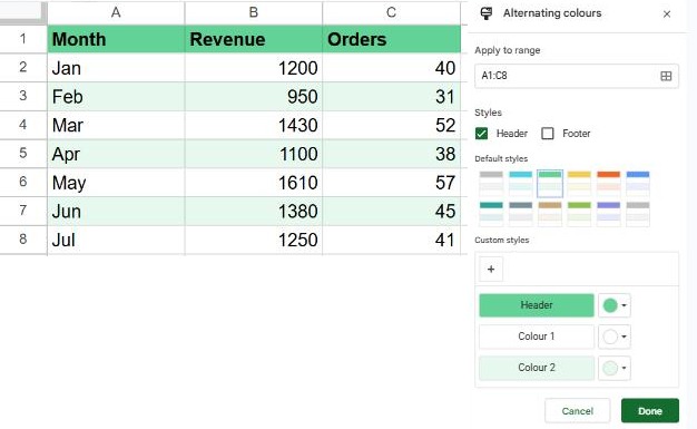
The stripes follow the data: if you sort, filter or insert rows, the pattern stays even.
Change or remove the colors
Click any cell in the table and open Format → Alternating colors again. Change the style, or click Remove alternating colors at the bottom of the panel.
Every other column, or groups of rows
The built-in tool only stripes rows one by one. For other patterns, use conditional formatting with a custom formula:
| Pattern | Custom formula |
|---|---|
| Every other column | =ISEVEN(COLUMN()) |
| Blocks of 3 rows | =ISEVEN(INT((ROW()-2)/3)) |
| Only rows with data | =AND($A1<>"", ISEVEN(ROW())) |
Frequently asked questions
Why can't I change the fill color of some cells?
Alternating colors sit underneath normal fill colors, so a cell you fill manually still shows your color. If nothing seems to change, check for a conditional formatting rule on the same range.
Does it work with filters?
Yes. Hidden or filtered rows don't break the pattern of the visible ones.
Is there a way to keep the header visible too?
Yes, freeze it. See how to freeze rows.