How to Transpose Data in Google Sheets (Rows to Columns)
Transposing flips a table on its side: rows become columns and columns become rows. It's handy when data arrives the "wrong way round", for example months listed down a column when you want them across the top.
Method 1: Paste special → Transposed
- Select the range you want to flip and copy it (Ctrl + C).
- Click the cell where the top-left corner of the result should go. Make sure there's enough empty space.
- Go to Edit → Paste special → Transposed, or right-click and choose Paste special → Transposed.
This pastes fixed values. If you change the original later, the transposed copy doesn't update.
Method 2: the TRANSPOSE function
To keep the flipped version linked to the original, type in an empty cell:
=TRANSPOSE(A1:C4)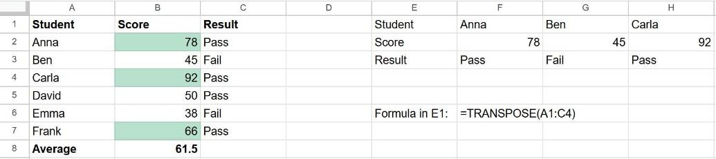
The result spills into as many cells as it needs: a range 4 rows tall and 3 columns wide becomes 3 rows tall and 4 columns wide.
Which method should you use?
| Paste special → Transposed | TRANSPOSE | |
|---|---|---|
| Updates when the source changes | No | Yes |
| You can edit the result cells | Yes | No (it's one formula) |
| Keeps formatting | Yes | No |
| Best for | One-off fixes | Live reports |
Frequently asked questions
Why does TRANSPOSE show #REF!?
Something is in the way of the result. Clear the cells where it needs to spill, below and to the right of the formula.
Can I edit a transposed cell?
Not with TRANSPOSE, because the whole area is one formula. Either edit the source, or copy the result and use Paste special → Values only to turn it into normal cells.
Do formulas survive a Paste special → Transposed?
Yes, but their cell references shift, which can break them. If the originals are formulas, pasting as values first is safer.