Fix "Did not find value in VLOOKUP evaluation" in Google Sheets
Your VLOOKUP returns #N/A, and when you hover over the cell Google Sheets says:
Error Did not find value 'P-101' in VLOOKUP evaluation.
The part in quotes is exactly what VLOOKUP searched for. If that value really isn't in your list, the error is correct. But if you can see it in the list, work through these checks in order. The first two explain most cases.
Check 1: did the range move when you copied the formula?
This is the classic one: the first rows work, and the error appears further down. You wrote this in F2 and dragged it down:
=VLOOKUP(E2, A2:C5, 3, FALSE)When you copy a formula, Sheets moves every reference with it. In F5 the formula has become =VLOOKUP(E5, A5:C8, 3, FALSE), so it only searches from row 5 down, and P-101 in row 2 is no longer in its range:
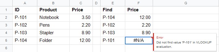
Fix: lock the range with dollar signs, so it stays put when copied, or use whole columns:
=VLOOKUP(E2, $A$2:$C$5, 3, FALSE)
=VLOOKUP(E2, A:C, 3, FALSE)
Click the range inside the formula and press F4 to add the dollar signs. More in absolute references explained.
Check 2: is the value in the first column of the range?
VLOOKUP only searches the first column of the range. With =VLOOKUP(E2, A2:C5, …) it looks in column A only. If your IDs are in column B, the range must start at B: B2:D5.
If the column you want to return is to the left of the search column, VLOOKUP can't do it. Use INDEX and MATCH or XLOOKUP instead.
Check 3: hidden spaces and invisible characters
"P-101" and "P-101 " (with a space at the end) look identical but don't match. Compare the lengths of the two cells:
=LEN(E5)
=LEN(A2)
If the numbers differ, there's an extra character. Remove normal spaces with Data → Data cleanup → Trim whitespace, or search with the trimmed value: =VLOOKUP(TRIM(E5), $A$2:$C$5, 3, FALSE). See how to remove extra spaces.
Data pasted from web pages sometimes contains non-breaking spaces, which trimming may not remove. Find out what the last character is with =CODE(RIGHT(A2)): 32 is a normal space, 160 a non-breaking one. Replace them with:
=SUBSTITUTE(A2, CHAR(160), "")Check 4: number on one side, text on the other
The number 101 and the text "101" are different values for VLOOKUP. It happens a lot with IDs, postcodes and data imported from other systems. Test both cells:
=ISNUMBER(E5)
=ISNUMBER(A2)
If one says TRUE and the other FALSE, convert one side. Either fix the data (see how to convert text to numbers) or convert the search key inside the formula:
=VLOOKUP(VALUE(E5), $A$2:$C$5, 3, FALSE)
=VLOOKUP(TO_TEXT(E5), $A$2:$C$5, 3, FALSE)
Use VALUE when the list holds numbers, and TO_TEXT when it holds text.
Check 5: the last argument
The fourth argument of VLOOKUP says whether the first column is sorted. If you leave it out, Google Sheets assumes TRUE (sorted) and does an approximate search. On data that isn't sorted, that gives #N/A or, worse, a wrong value.
Fix: unless you're doing a deliberate range lookup (like tax brackets), always end with FALSE.
Check 6: the value really isn't there
Press Ctrl+F and search for the value from the message. If it isn't in the list, the error is correct, and you can show something friendlier instead:
=IFNA(VLOOKUP(E5, $A$2:$C$5, 3, FALSE), "Not found")Why IFNA and not IFERROR is explained in how to fix the #N/A error.
Same message in MATCH and HLOOKUP
MATCH and HLOOKUP give the same kind of message, for example "Did not find value 'P-101' in MATCH evaluation." The checks are the same. For HLOOKUP, check 2 applies to the first row of the range instead of the first column.
Frequently asked questions
Is VLOOKUP case-sensitive?
No. "p-101" finds "P-101". Upper and lower case are never the reason for this error.
Why does it work in some rows and not others?
Almost always check 1: the range moved when the formula was copied down. Lock it with $.
Can I search in another tab or file?
Yes. See VLOOKUP from another sheet. For another file, combine it with IMPORTRANGE.
How do I quickly test if two cells are the same?
Type =E5=A2. If it says FALSE when both look identical, the difference is a space, an invisible character or number vs text: checks 3 and 4.