How to VLOOKUP from Another Sheet in Google Sheets

Most real spreadsheets keep lookup tables on their own tab, like a Products list or a price list. VLOOKUP can search a different tab by putting the tab name in front of the range.

The syntax

=VLOOKUP(search_key, SheetName!range, column, FALSE)

The only difference from a normal VLOOKUP is SheetName! before the range: the tab name followed by an exclamation mark.

Example

An Orders tab lists product IDs in column B. The prices live on a tab called Products, with IDs in column A and prices in column C. In C2 of the Orders tab:

=VLOOKUP(B2, Products!A2:C5, 3, FALSE)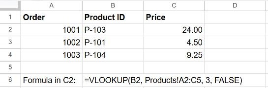

VLOOKUP in Google Sheets pulling prices from a separate Products tab — Each order gets its price from the Products tab.

You don't have to type the tab name: after =VLOOKUP(B2, , click the Products tab, select the range with the mouse, and Sheets fills in Products!A2:C5 for you. Then finish the formula and press Enter.

Tab names with spaces

If the tab name contains spaces or symbols, wrap it in single quotes:

=VLOOKUP(B2, 'Price list'!A2:C50, 3, FALSE)

Copying the formula down

Lock the range with $ so it doesn't slide as you fill down, or use whole columns:

=VLOOKUP(B2, Products!$A$2:$C$50, 3, FALSE)
=VLOOKUP(B2, Products!A:C, 3, FALSE)

See absolute references.

From a different file

To look up data in another spreadsheet file, combine VLOOKUP with IMPORTRANGE:

=VLOOKUP(B2, IMPORTRANGE("spreadsheet_url", "Products!A2:C50"), 3, FALSE)

The first time, Sheets asks you to allow access between the two files. More in how to use IMPORTRANGE.

Frequently asked questions

Why do I get #REF!?

Usually the tab name is misspelled, has spaces but no quotes, or was renamed. Also check that the column number isn't larger than the range. See how to fix #REF!.

Why do I get #N/A?

The ID isn't found in the first column of the range, often because of extra spaces. See how to fix #N/A.