How to Use the IF Function in Google Sheets (With Examples)
The IF function lets a cell make a decision: if a condition is true, show one thing; if it's false, show another. It's how you turn a column of numbers into "Pass" and "Fail", flag overdue invoices, or apply a discount only above a certain amount.
IF syntax
=IF(logical_expression, value_if_true, value_if_false)- logical_expression – a test that is either TRUE or FALSE, such as
B2>=50. - value_if_true – what the cell shows when the test is TRUE.
- value_if_false – what the cell shows when the test is FALSE. If you leave it out, the cell shows FALSE.
Example: pass or fail
A class list has student names in column A and scores in column B. Anyone with 50 or more passes. In cell C2, type:
=IF(B2>=50, "Pass", "Fail")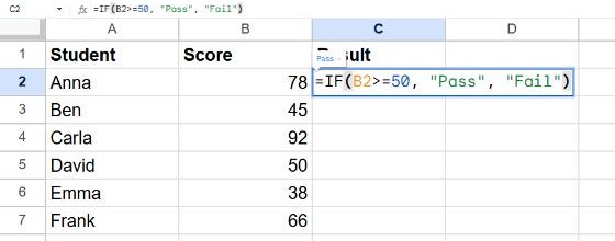
Press Enter, then copy the formula down to the other rows. The quickest way: select C2 down to the last row and press Ctrl + D (⌘ + D on Mac).
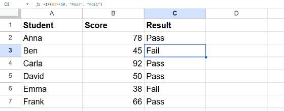
>= means "greater than or equal to".Remember the quotes: text results like "Pass" must be in double quotes. Numbers and cell references don't need them.
Comparison operators you can use
| Operator | Meaning | Example |
|---|---|---|
= | Equal to | A2="Paid" |
<> | Not equal to | A2<>"Paid" |
> | Greater than | B2>100 |
< | Less than | B2<0 |
>= | Greater than or equal to | B2>=50 |
<= | Less than or equal to | B2<=10 |
Text comparisons are not case-sensitive: A2="paid" is TRUE when A2 contains "Paid".
Return a calculation instead of text
The true and false values can be formulas. For example, give a 10% discount on orders of 100 or more:
=IF(B2>=100, B2*0.9, B2)Leave the cell empty
Use two double quotes with nothing between them to show a blank. This is handy to avoid results in rows that have no data yet:
=IF(B2="", "", IF(B2>=50, "Pass", "Fail"))Several conditions: nested IF and IFS
To give letter grades, you can put one IF inside another:
=IF(B2>=90, "A", IF(B2>=70, "B", IF(B2>=50, "C", "F")))Sheets checks the conditions in order and stops at the first one that is TRUE. Nested IFs get hard to read, so Google Sheets also offers IFS, which takes pairs of condition and result:
=IFS(B2>=90, "A", B2>=70, "B", B2>=50, "C", TRUE, "F")The final TRUE, "F" acts as "everything else". Without it, IFS returns an error when no condition matches.
Combine IF with AND or OR
- AND – all conditions must be true. Pass only if both the exam (B2) and the project (C2) are 50 or more:
=IF(AND(B2>=50, C2>=50), "Pass", "Fail") - OR – at least one condition must be true. Flag an order if it's urgent or over 500:
=IF(OR(D2="Urgent", E2>500), "Check", "")
Frequently asked questions
Why does my IF formula return #ERROR!?
Usually a missing quote or bracket. Check that every text value has opening and closing double quotes and that the number of ( matches the number of ).
Can I check whether a cell contains a word?
Yes, combine IF with REGEXMATCH or SEARCH. For example, =IF(ISNUMBER(SEARCH("refund", A2)), "Refund", "") finds "refund" anywhere in the text, ignoring case.
How do I count how many rows passed?
Use COUNTIF on the result column: =COUNTIF(C2:C7, "Pass"). See our COUNTIF guide for more examples.