How to Fix "Formula parse error" (#ERROR!) in Google Sheets
When a cell shows #ERROR! and the tooltip says Formula parse error, Google Sheets couldn't even read your formula. It's a typing problem, not a data problem: a character is missing, extra or not the one Sheets expects. Here are the usual culprits, from most to least common.
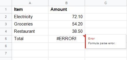
Quick reference:
| Causes the error | Works |
|---|---|
=IF(B2>50, "High", "Low") in a Spanish, German or French sheet | =IF(B2>50; "High"; "Low") |
=IF(B2>50, “Very high”, “OK”) | =IF(B2>50, "Very high", "OK") |
=IF(B2>50, Very high, "OK") | =IF(B2>50, "Very high", "OK") |
=SUM(B2:B4)) | =SUM(B2:B4) |
=SUM(Sales 2026!B2:B4) | =SUM('Sales 2026'!B2:B4) |
=B2 B3 or =B2*/B3 | =B2*B3 |
=B5*1,000 | =B5*1000 |
1. Commas or semicolons?
This is the big one, especially if you copied a formula from a website or a tutorial. Google Sheets separates function arguments with commas in some countries and with semicolons in others. It depends on the spreadsheet's locale:
- Commas
,: United States, United Kingdom, Mexico, India and other countries that write decimals with a point (3.5). - Semicolons
;: Spain, Germany, France, Italy, Brazil and other countries that write decimals with a comma (3,5).
If your sheet expects semicolons and you type =IF(B2>50, "High", "Low"), you get a parse error. Replace each comma between arguments with a semicolon: =IF(B2>50; "High"; "Low").
To check or change it, go to File → Settings and look at Locale on the General tab. Changing the locale also changes how dates, numbers and currencies are shown, so it's usually easier to adapt the formula.
The same rule applies to { } arrays: in semicolon locales, columns are separated with a backslash, so {1, 2, 3} becomes {1 \ 2 \ 3}.
2. Curly quotes
Formulas copied from Word, Google Docs, a chat or some websites often come with typographic quotes “ ” instead of straight ones " ". They look almost identical, but Sheets only understands the straight ones, so it treats the text as if it had no quotes at all. That gives a parse error, or #NAME? when the text is a single word (see the next section).
Fix: click the cell, delete each quote in the formula bar and type it again from your keyboard. If there are many, use Find and replace with Also search within formulas ticked: replace “ with ", then ” with ".
3. Text without quotes
Text inside a formula must be in double quotes. Without them, a phrase with spaces such as Very high can't be read and gives a parse error. A single word without quotes gives #NAME? instead, because Sheets thinks it's the name of a range.
Fix: wrap every piece of text in straight double quotes: "Very high". Numbers, cell references and TRUE/FALSE don't need quotes.
4. Brackets that don't match
Every ( needs its own ). An extra closing bracket, as in =SUM(B2:B4)), or one in the wrong place in a nested formula, makes the formula unreadable.
Fix: count the brackets. With nested IFs it helps to write the formula on several lines: press Ctrl+Enter (⌘+Enter on Mac) inside the formula bar to add a line break, so each IF sits on its own line.
5. Sheet names with spaces
When you refer to another tab whose name contains spaces or symbols, the name must be in single quotes:
=SUM('Sales 2026'!B2:B4)Without them (=SUM(Sales 2026!B2:B4)) you get a parse error. The easiest way to get it right is not to type it: start the formula, then click the other tab and select the cells. Sheets writes the reference, quotes included.
6. Missing or doubled operators
Between two values there must be exactly one operator: + - * / ^ &.
=B2 B3(no operator) and=2(B2+B3)(no*before the bracket) don't work. Write=B2*B3and=2*(B2+B3).=B2*/B3has two operators in a row. Remove one.- To join text, use
&:=A2&" "&B2. See how to combine text.
7. Numbers with thousands separators
Inside a formula, type numbers without thousands separators or currency symbols. =B5*1,000 or =B5*€20 can't be read; use =B5*1000 and =B5*20. Format the result as currency afterwards with Format → Number.
Frequently asked questions
What's the difference between #ERROR! and the other errors?
#ERROR! means Sheets couldn't read the formula at all. The others mean it read the formula but something went wrong when calculating: #NAME? for an unknown name, #VALUE! for the wrong type of data, #N/A for a lookup that found nothing, and #REF! for a broken reference.
Can IFERROR hide a parse error?
No. A formula that can't be read never runs, so IFERROR never gets a chance to catch anything. You have to fix the formula itself.
The formula works in Excel or in another file. Why not here?
Almost always it's the locale: the other file uses commas and this one semicolons, or the other way round. Check File → Settings → Locale in both files.
Why does my IMPORTRANGE give #ERROR!?
Both arguments must be text in double quotes: the file URL and the range, for example "Sheet1!A1:C10". See how to use IMPORTRANGE.