Fix #NUM! in Google Sheets: 8 Causes and Their Fixes

#NUM! means the formula is fine, but a number in it isn't valid for that function: a negative square root, a position that doesn't exist, a start date after the end date, or a result too big to store. Hover over the cell and Sheets tells you exactly which one. We triggered every common case in a real sheet:

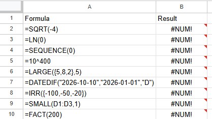
Google Sheets with nine formulas in column A, such as =SQRT(-4), =LN(0) and =FACT(200), all returning #NUM! in column B — Nine different formulas, one error. The tooltip is what tells them apart.

Find the message from your tooltip below.

"Function SQRT parameter 1 value is negative"

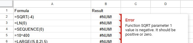
A square root of a negative number doesn't exist as a regular number, so =SQRT(-4) fails. It usually happens when the cell inside SQRT is a difference that turned negative.

Fix: if only the size matters, take the absolute value first. If a negative value means the data is wrong, leave the cell blank instead:

=SQRT(ABS(A2))
=IF(A2<0, "", SQRT(A2))

"Function LN parameter 1 value is 0"

=LN(0) shows "Function LN parameter 1 value is 0. It should be greater than 0." Logarithms (LN, LOG, LOG10) only work with numbers above zero, and an empty cell counts as 0.

Fix: only calculate when the value is positive:

=IF(A2>0, LN(A2), "")

"Function LARGE parameter 2 value 5 is out of range"

=LARGE({5,8,2}, 5) asks for the 5th largest value in a list of only three. SMALL works the same way.

Fix: make sure the position is between 1 and the number of values. For a "top 5" list that may have fewer rows, return a blank when the position doesn't exist:

=IFERROR(LARGE(B2:B20, 5), "")

In our test, this formula returned an empty cell instead of the error.

"SMALL has no valid input data"

=SMALL(D1:D3, 1) on an empty range gives "SMALL has no valid input data." Either the range is empty, or the numbers in it are stored as text, which these functions ignore.

Fix: check that the range points to the right cells. If the values are left-aligned, they're probably text: see how to convert text to numbers.

"Function DATEDIF parameter 1 … should be on or before Function DATEDIF parameter 2"

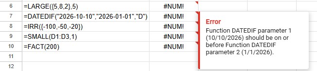
Google Sheets tooltip: Function DATEDIF parameter 1 (10/10/2026) should be on or before Function DATEDIF parameter 2 (1/1/2026). — The start date (10/10/2026) is after the end date (1/1/2026).

DATEDIF needs the earlier date first. It's the most common #NUM! in date sheets: two columns swapped, or a deadline that has already passed.

Fix: put the start date first. If you don't know which date comes first, let MIN and MAX order them:

=DATEDIF(MIN(A2, B2), MAX(A2, B2), "D")

With the dates from the screenshot this returned 282 days. If you need negative results for past dates, skip DATEDIF and subtract instead: =B2-A2. More in how to count days between dates.

"Function SEQUENCE parameter 1 value is 0"

=SEQUENCE(0) shows "Function SEQUENCE parameter 1 value is 0. It should be greater than or equal to 1." It happens when the number of rows comes from another formula, like =SEQUENCE(COUNTA(A2:A)), and the list is still empty.

Fix: return a blank when the count is 0, or force at least one row:

=IF(COUNTA(A2:A)=0, "", SEQUENCE(COUNTA(A2:A)))
=SEQUENCE(MAX(1, COUNTA(A2:A)))

"Numeric value is greater than 1.79769E+308"

=10^400 shows "Numeric value is greater than 1.79769E+308 and cannot be displayed properly." That's the largest number Google Sheets can store. FACT has its own, lower limit: =FACT(200) says "Function FACT parameter 1 value is 200. It should be less than or equal to 170."

Fix: a result this big almost always means a wrong reference, for example an exponent pointing at a year (2026) instead of a number of years. Check the cells the formula uses. If you really work with huge numbers, compare their logarithms (LOG10) instead.

"In IRR evaluation, the value array must include positive and negative numbers"

=IRR({-100,-50,-20}) fails because there's money going out but nothing coming back. IRR needs at least one negative value (the investment) and one positive value (a return).

Fix: check the signs of your cash flows. Payments should be negative and income positive. =IRR({-100,60,70}) returned 19% in our test.

Hide #NUM! with IFERROR

Here are the fixes from this guide, tested in the same sheet:

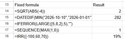
Fixed formulas in Google Sheets: SQRT(ABS(-4)) returns 2, DATEDIF with MIN and MAX returns 282, IFERROR(LARGE(...)) returns blank, SEQUENCE(MAX(1,0)) returns 1, IRR returns 19% — No more #NUM!: each formula handles the invalid case.

If you just want a clean report, =IFERROR(your_formula, "") hides the error. Use it with care: it also hides every other error, so a typo or a broken reference will silently show a blank too. See how to use IFERROR.

Frequently asked questions

What's the difference between #NUM! and #VALUE!?

#VALUE! means the function got the wrong type of data, like text where it expected a number. #NUM! means it got a number, but one that's impossible for that calculation. See how to fix #VALUE!.

Why do I get #NUM! with a formula that worked yesterday?

The formula didn't change, the data did: a date passed (DATEDIF), a list became empty (SEQUENCE, SMALL), or a value turned negative (SQRT). Hover over the cell to see which input broke it.