How to Use IFERROR in Google Sheets (with Examples)
IFERROR checks whether a formula returns an error. If it does, it shows a value you choose instead; if it doesn't, it shows the normal result. It's the quickest way to keep a sheet clean when some rows are expected to fail, such as lookups for items that aren't in a list yet.
The syntax
=IFERROR(value, [value_if_error])- value: the formula you want to protect.
- value_if_error: what to show if it fails. If you leave it out, Sheets shows an empty cell.
Example
A price per unit is calculated as =B2/C2. When the quantity is 0, the result is #DIV/0!. Wrapped in IFERROR, the error disappears:
=IFERROR(B2/C2, "-")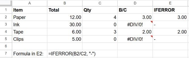
Common uses
| Situation | Formula |
|---|---|
| Lookup that may not find a match | =IFERROR(VLOOKUP(E2, A2:C20, 3, FALSE), "Not found") |
| Division that may be by zero | =IFERROR(B2/C2, 0) |
| Average of a range that may be empty | =IFERROR(AVERAGE(B2:B20), "") |
IFERROR vs IFNA
IFERROR catches every error: #N/A, #DIV/0!, #VALUE!, #REF! and #NAME?. That's convenient but risky: a typo in a function name or a deleted column would also be hidden, and you'd never notice the formula is broken.
For lookups, IFNA is safer because it only catches "not found":
=IFNA(VLOOKUP(E2, A2:C20, 3, FALSE), "Not found")Rule of thumb: build and test the formula first, and only wrap it in IFERROR once you know it works. Otherwise you'll hide the very errors that tell you what's wrong.
Frequently asked questions
Can I show a blank instead of an error?
Yes: =IFERROR(B2/C2, ""), or simply =IFERROR(B2/C2) with no second argument.
Does IFERROR slow down my sheet?
Not noticeably. It only evaluates the formula once.
Why is my IFERROR still showing an error?
Check the brackets: the whole formula must be inside IFERROR's first argument. =IFERROR(B2)/C2 protects B2, not the division.