How to Use the RANK Function in Google Sheets

RANK tells you where a number stands in a list: 1st, 2nd, 3rd and so on. It's handy for leaderboards, top sellers or class results.

The syntax

=RANK(value, data, [is_ascending])

value: the number to rank.
data: the whole list of numbers. Lock it with $ so it doesn't move when you fill down.
is_ascending (optional): leave it out or use 0 for highest = 1; use 1 for lowest = 1 (for example race times).

Example

=RANK(B2, $B$2:$B$7)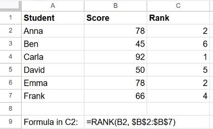

RANK function in Google Sheets ranking six student scores, with two students tied in 2nd place — Anna and Emma both scored 78, so both are ranked 2 and the next rank is 4.

See absolute references if you're not sure why the range has dollar signs.

How ties work

Equal values get the same rank, and the next rank is skipped (1, 2, 2, 4). If you'd rather give tied values the average rank (2.5 each), use RANK.AVG instead. RANK.EQ behaves exactly like RANK.

Break ties

To give every row a unique rank, add a tiny tie-breaker based on the row order:

=RANK(B2, $B$2:$B$7) + COUNTIF($B$2:B2, B2) - 1

The first 78 stays 2nd and the second becomes 3rd.

Rank within a group

To rank each student only within their class (class in column A), count how many in the same class scored higher:

=COUNTIFS($A$2:$A$20, A2, $B$2:$B$20, ">"&B2) + 1

Frequently asked questions

Why does RANK return #N/A?

The value isn't in the data range, often because the range moved when you filled the formula down. Add the $ signs.

How do I sort by rank?

Sort the table by the rank column, or directly by the score. See how to sort data.